Periodic Costing Use Methods and Modes
Periodic Costing includes two costing methods and two modes.
Periodic Costing calculates the cost of items periodically and generates GL transactions according to the period costs for all costs, using one of two methods:
• Weighted Average (WAVG)
WAVG considers the previous period cost and the average of the cost incurred during this period.
• First in First Out (FIFO)
FIFO considers the receipt date of items for the existing inventory and assumes that the oldest (first) receipts in stock of the item are issued first.
For more information on WAVG and FIFO, refer to
Periodic Costing Methods.
For modes, you can set up Periodic Costing in either of two modes:
• Adjustment mode
• Complete mode
The following topics explain the two modes in more detail.
Adjustment Mode
Customers who have requirements to produce financial reports based on both standard cost and Periodic Cost (WAVG or FIFO) should use the adjustment mode for Periodic Costing.
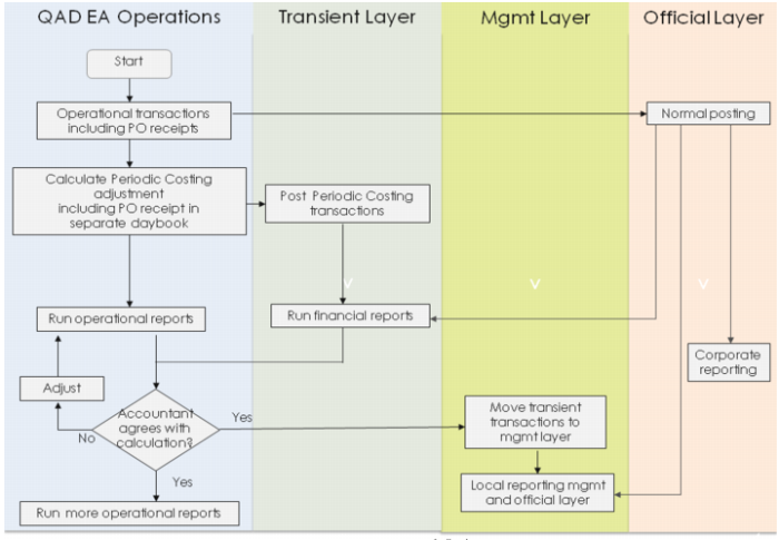
For this purpose, the system makes use of the layers concept in GL. The system posts standard cost transactions to the official layer, and it posts the periodic cost transactions to the transient and management layer once the period closes. Corporate reporting is through the official layer and local reporting is through a combination of the management and official layers.
Adjustment mode means that the operational module generates GL transactions at the standard cost at the same time as the transaction happens. The Periodic Costing calculation then revalues all of these transactions and creates adjustment GL transactions.
When you use adjustment mode, you have instantaneous costing data from standard costs. The system creates general ledger transactions when you create inventory transactions. It creates period cost transactions at the end of the period. You set Create GL Transactions to Yes in Inventory Accounting Control (36.9.2).
Multinational companies can use standard costing to meet their management accounting, internal audit, and corporate requirements, while also using Periodic Costing functions for legal (end of period) accounting or actual costs requirements.
Periodic Cost calculation uses an adjustment method that ensures accurate calculations. The adjustment logic begins by fully reversing the original transactions and then recalculating the PC GL transactions using the full amount to post the transactions to the accounts.
When you use adjustment mode, you can make analysis on inventory valuation based on both standard cost and the calculated periodic costs.
C Periodic Costing, Adjustment Mode Flow present a flowchart for the adjustment mode calculations.
C
Periodic Costing, Adjustment Mode Flow
Complete Mode
In complete mode, the system does not post any standard cost transactions. It only posts periodic inventory costs to the GL at the end of the period. As opposed to adjustment mode, the complete mode only produces one type of financial book based on periodic cost.
In this mode, you set Create GL Transactions to No in Inventory Accounting Control (36.9.2). In this mode, the system continues to post PO receipts transactions. This is required so that AP sub-ledger accounts always match correctly, without having to wait until the Periodic Costing close process posts to the GL.
Complete mode is less frequently in use, although in Brazil and in certain other locales, it may be a preferred best practice. Typically, complete mode is used by local companies operating in locations where standard costing is prohibited.
In complete mode, there will only be Periodic Cost based transactions calculated at the end of the period. These transactions are posted to the transient layer. Once the period is closed, the PC transactions are moved from the transient to the official layer. The following graphic depicts the flow for GL posting, using the complete mode.
Periodic Costing Methods
Two methods for periodic costing are available:
For WAVG, you can determine the item unit cost by analyzing initial inventory before period start as all received inventory during the calculation period, but for FIFO, item unit cost is based on how inventory is consumed. For more information, see
Weighted Average (WAVG).
For FIFO, there are key differences in theoretical calculations and the QAD approach. The QAD approach approximates the theoretical calculations but considers practical issues such as:
• The number of daily transactions, which can be very large
• The large number of users for which transaction sequencing can be cumbersome
• Asynchronous physical receipts or issues versus data captured
• Complexities when calculating production transactions
Also, when you use FIFO, for the overhead cost of RCT-PO, you set up overhead cost of the prior period using PC Unit Cost Adjustment. When the system processes RCT-PO, it reads the PC cost from the prior period cost set.
For FIFO, when there are multiple buckets set up for every period, you should set up overhead cost for the first bucket of prior period. For more information on FIFO, see
First, In, First Out (FIFO).
In the QAD solution, the system averages the unit costs by cost calculation period, by dividing total value of received goods by the total quantity received. The system maintains the quantity received by cost calculation period by consuming the inventory from the oldest periods first and then chronologically period by period up to the most recent period.
The topics within this section explain each method and provide examples in tables. In the tables, goods for sale (or quantity to issue) considers the beginning inventory and the quantities received during that period, which are the inbound receipt transactions. The different formulas to define the periodic costs are illustrated using the example shown in
Formula Example.
Formula Example
Beginning Balance | Qty QOH | Unit Cost | Value |
| 300 | 2 | 600 |
| | | |
Receipts | Qty Received | Unit Cost | Value |
May 1 | 200 | 2.2 | 440 |
May 8 | 300 | 2.3 | 690 |
May 14 | 200 | 2.5 | 500 |
Total Received | 700 | | 1630 |
| | | |
Goods for Sale | 1000 | | 2230 |
| | | |
Issues | Qty Issued | Unit Cost | Value |
May 8 | -150 | | |
May 22 | -200 | | |
May 28 | -400 | | |
Total Issued | -750 | | |
| | | |
End Balance | QTY OH | Unit Cost | Value |
| 250 | | |
Weighted Average (WAVG)
Weighted average (WAVG) considers the previous period cost and the average of the cost incurred this period. WAVG assumes that the material or production of a given kind is so intermingled that an issue cannot be made from a particular lot and cost should, therefore, represent an average of the entire supply. The calculation considers the previous period cost and the average of the cost incurred this period. The system looks at the Inventory and WIP Balance Report (30.5.19.2) to determine the ending balance from location detail and uses the information when determining costs in the cost calculation period when you use the WAVG method.
Average cost produces results that typically fall somewhere between results for FIFO costs. The calculation is as follows:
This period material cost = (Sum of this period (receipt quantity * receipt cost) / (this period receipt quantity)
Note: You define the period using PC Periods Maintenance (30.5.1.1).
Received Quantity | Unit Cost at Receipt |
200 | 2.20 |
300 | 2.30 |
200 | 2.50 |
This period material cost = (200 * 2.20 +300 * 2.30 + 200 * 2.50) / (200 + 300 + 200) = 2.33
The unit cost calculation is as follows:
(This period material cost * this period receipt quantity + last period unit cost * last period item quantity balance + this period material cost adjustment) / (this period receipt quantity + last period item quantity balance)
Opening Inventory Balance | Last Period Unit Cost |
300 | 2.00 |
This period unit cost = (700 * 2.33 + 300 * 2.00) / (700 + 300) = 2.23
For the following examples, WAVG is in use to define the periodic costs using the example shown in
Formula Example.
WAVG Example
Beginning Balance | Qty QOH | Unit Cost | Value |
| 300 | 2 | 600 |
| | | |
Receipts | Qty Received | Unit Cost | Value |
May 1 | 200 | 2.2 | 440 |
May 8 | 300 | 2.3 | 690 |
May 14 | 200 | 2.5 | 500 |
Total Received | 700 | | 1630 |
| | | |
Goods for Sale | 1000 | | 2230 |
| | | |
Issues | Qty Issued | Unit Cost | Value |
May 8 | -150 | | |
May 22 | -200 | | |
May 28 | -400 | | |
Total Issued | -750 | | |
| | | |
End Balance | QTY OH | Unit Cost | Value |
| 250 | | |
Average cost produces results that typically fall somewhere between results for FIFO. The calculation is as follows:
This period material cost = (Sum of this period (receipt quantity * receipt cost) / (this period receipt quantity)
Note: You define the period using PC Periods Maintenance (30.5.1.1).
Received Quantity | Unit Cost at Receipt |
200 | 2.20 |
300 | 2.30 |
200 | 2.50 |
This period material cost = (200 * 2.20 +300 * 2.30 + 200 * 2.50) / (200 + 300 + 200) = 2.33
The unit cost calculation is as follows:
(This period material cost * this period receipt quantity + last period unit cost * last period item quantity balance + this period material cost adjustment) / (this period receipt quantity + last period item quantity balance)
Opening Inventory Balance | Last Period Unit Cost |
300 | 2.00 |
This period unit cost = (700 * 2.33 + 300 * 2.00) / (700 + 300) = 2.23
WAVG Example
Beginning Balance | Qty QOH | Unit Cost | Value |
| 300 | 2 | 600 |
| | | |
Receipts | Qty Received | Unit Cost | Value |
May 1 | 200 | 2.2 | 440 |
May 8 | 300 | 2.3 | 690 |
May 14 | 200 | 2.5 | 500 |
Total Received | 700 | 2.32857 | 1630 |
| | | |
Goods for Sale | 1000 | 2.23 | 2230 |
| | | |
Issues | Qty Issued | Unit Cost | Value |
May 8 | -150 | 2.23 | -334.5 |
May 22 | -200 | 2.23 | -446 |
May 28 | -400 | 2.23 | -892 |
Total Issued | -750 | 2.23 | -1672.5 |
| | | |
End Balance | QTY OH | Unit Cost | Value |
| 250 | 2.23 | 557.5 |
First, In, First Out (FIFO)
The First In, First Out (FIFO) method considers the receipt date of items for all existing inventory. This method assumes that the oldest (first) item in stock is issued first.
For FIFO, there are key differences in theoretical calculations and the QAD approach. The QAD approach approximates the theoretical calculations but considers practical issues such as:
• The number of daily transactions, which can be very large
• The large number of users for which transaction sequencing can be cumbersome
• Asynchronous physical receipts or issues versus data captured
• Complexities when calculating production transactions
In the QAD solution, the system averages the unit costs by cost calculation period, by dividing total value of received goods by the total quantity received. The system maintains the quantity received by cost calculation period by consuming the inventory from the oldest periods first and then chronologically period by period up to the most recent period.
Also, when you use FIFO, for the overhead cost of RCT-PO, you set up overhead cost of the prior period using PC Unit Cost Adjustment. When the system processes RCT-PO, it reads the PC cost from prior period cos set.
For FIFO, when there are multiple buckets set up for every period, you should set up overhead cost for the first bucket of prior period.
The following table provides the theoretical way that FIFO is calculated.
FIFO Theoretical Example
Beginning Balance | Qty QOH | Unit Cost | Value | |
| 300 | 2 | 600 | |
| | | | |
Receipts | Qty Received | Unit Cost | Value | |
May 1 | 200 | 2.2 | 440 | |
May 14 | 300 | 2.3 | 690 | |
May 31 | 200 | 2.5 | 500 | |
Total Received | 700 | 2.33 | 1630 | |
| | | | |
Goods for Sale | 1000 | | 2230 | |
| | | | |
Issues | Qty Issued | Unit Cost | Value | Value Calculations |
May 8 | -150 | | -300 | (150 * 2) Initial inventory |
May 22 | -200 | | -410 | (150*2 + 50*2.2) Remaining initial inventory and receipt of 50 on May 1. |
May 28 | -400 | | -906 | (150*2.2 + 250*2.3) |
Total Issued | -750 | | -710 | |
| | | | |
End Balance | QTY OH | Unit Cost | Value | |
| 250 | 2.34 | 615 | |
Beginning Balance | 0 | 2 | 0 | |
May 1 | 0 | 2.2 | 0 | |
May 14 | 50 | 2.3 | 115 | |
May 31 | 200 | 2.5 | 500 | |
The ending inventory was received at two occasions’ costs:
Quantity | Receipt Unit Cost |
50 Remaining stock received May 14 | 2.3 |
200 Remaining stock received May 31 | 2.5 |
Ending inventory value: 50 * 2.3 + 200 * 2.5 = 615
Unit cost: 615 / 250 = 2.46
The FIFO method provides a good indication of the balance sheet value of ending inventory. However, in an economy with rising prices, it also increases net income because older inventory is used to value the cost of goods sold—potentially increasing the amount of taxes that a company should pay.
The following example shows the QAD FIFO solution.
FIFO QAD Solution
Beginning Balance | Qty QOH | Unit Cost | Value | |
| 300 | 2 | 600 | |
| | | | |
Receipts | Qty Received | Unit Cost | Value | |
May 1 | 200 | 2.2 | 440 | |
May 14 | 300 | 2.3 | 690 | |
May 31 | 200 | 2.5 | 500 | |
Total Received
Bucket 1 | 700 | 2.32857 | 1630 | |
Goods for Sale | 1000 | | 2230 | |
| | | | |
Issues | Qty Issued | Unit Cost | Value | Value Calculations |
May 8 | -150 | | -300 | (150 * 2) |
May 22 | -200 | | -416.3 | (400*2.32857) |
May 28 | -400 | | -931.43 | (400*2.32857) |
Total Issued | -750 | | -710 | |
| | | | |
End Balance | QTY OH | Unit Cost | Value | |
| 250 | 2.32857 | 582.14 | |
Beginning Balance | 0 | 2 | 0 | |
Balance Bucket 1 | 250 | 2.32857 | 582.14 | |
The QAD FIFO solution considers buckets with a weighted average that is calculated based on all receipts and specific related costs.
In the example, the system created only one bucket. The system first calculates the weighted average of the bucket; then, consumes inventory based on FIFO principles.
Note: The smaller the buckets, the closer the QAD FIFO value approximates the theoretical FIFO value; however, it makes the system more difficult to maintain and periodic costing calculations longer. So, it is a business consideration to decide the number of buckets to define by GL calendar period. For example, having two buckets (one from May 1-15 and the other from May 16-31) causes two unit cost values (2.26 for the first bucket and 2.5 for the second bucket) to be calculated.
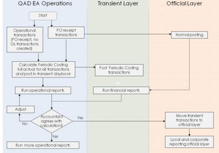 GL Posting Flow, Complete Mode