Operations Planning Example
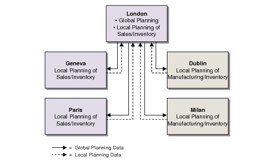
Planning Relationships shows the operations planning relationships between sites. In addition to marketing, London is the central site for operations planning. Each of the other four sites plans its own activities, then provides the local planning data to the London master scheduler.
Planning Relationships
The London scheduler consolidates this data and calculates a weekly global operations plan for each product. This plan shows consolidated sales forecasts, target inventory levels, and production due.
London then distributes the global plan to all sites. The local site planners transform this plan into weekly production schedules.
In
Global Sales Forecasts for London, London calculates a global operations plan. London, Geneva, and Paris generate sales forecasts. Milan and Dublin provide inventory required to satisfy these forecasts. London calculates global sales forecasts by consolidating its own forecasts with those from Geneva and Paris.
Global Sales Forecasts for London
Week | Geneva Forecasts | Paris Forecasts | Global Forecasts |
1 | 0 | 0 | 0 |
2 | 4,000 | 6,000 | 4,000 + 6,000 = 10,000 |
3 | 7,000 | 5,000 | 7,000 + 5,000 = 12,000 |
4 | 4,500 | 6,500 | 4,500 + 6,500 = 11,000 |
5 | 4,500 | 4,500 | 4,500 + 4,500 = 9,000 |
6 | 5,000 | 5,000 | 5,000 + 5,000 = 10,000 |
7 | 6,000 | 5,000 | 6,000 + 5,000 = 11,000 |
8 | 6,000 | 6,000 | 6,000 + 6,000 = 12,000 |
9 | 8,000 | 5,000 | 8,000 + 5,000 = 13,000 |
London calculates global target inventory levels to support the next two weeks of sales forecasts from London, Geneva, and Paris. Therefore, the target inventory level is the total global forecast for the next two weeks.
Global Forecasts and Target Inventory Levels for London
Week | Global Forecasts | Global Target Inventory Levels |
1 | 0 | 10,000 + 12,000 = 22,000 |
2 | 10,000 | 12,000 + 11,000 = 23,000 |
3 | 12,000 | 11,000 + 9,000 = 20,000 |
4 | 11,000 | 9,000 + 10,000 = 19,000 |
5 | 9,000 | 10,000 + 11,000 = 21,000 |
6 | 10,000 | 11,000 + 12,000 = 23,000 |
7 | 11,000 | 12,000 + 13,000 = 25,000 |
8 | 12,000 | 13,000 + 0 = 13,000 |
9 | 13,000 | 0 |
Production due is the consolidated production requirement, calculated with the following formula.
(Sales Forecast + Target Inventory) – Previous Week’s Projected Quantity on Hand
For week 1, the projected quantity on hand is the ending inventory balance from the previous week (or 3,000, in this example). For weeks 2 to 9, projected quantity on hand equals the target inventory level for the previous week.
Production Calculations
Wk | Forecasts | Target Inv | Prev QOH | Global Production Due |
1 | 0 | 22,000 | 3,000 | (0 + 22,000) – 3,000 = 19,000 |
2 | 10,000 | 23,000 | 22,000 | (10,000 + 23,000) – 22,000 = 11,000 |
3 | 12,000 | 20,000 | 23,000 | (12,000 + 20,000) – 23,000 = 9,000 |
4 | 11,000 | 19,000 | 20,000 | (11,000 + 19,000) – 20,000 = 10,000 |
5 | 9,000 | 21,000 | 19,000 | (9,000 + 21,000) – 19,000 = 11,000 |
6 | 10,000 | 23,000 | 21,000 | (10,000 + 23,000) – 21,000 = 12,000 |
7 | 11,000 | 25,000 | 23,000 | (11,000 + 25,000) – 23,000 = 13,000 |
8 | 12,000 | 13,000 | 25,000 | (12,000 + 13,000) – 25,000 = 0 |
9 | 13,000 | 0 | 13,000 | (13,000 + 0) – 13,000 = 0 |
London will use the operations plan to view the global picture of sales forecasts, target inventory, and production due for this item. Milan and Dublin will use it for site-level planning, scheduling, and manufacturing activities.
Production Calculations and Projected Quantities on Hand
Wk | Forecasts | Target Inventory | Production Due | Projected QOH |
1 | 0 | 22,000 | 19,000 | 22,000 |
2 | 10,000 | 23,000 | 11,000 | 23,000 |
3 | 12,000 | 20,000 | 9,000 | 20,000 |
4 | 11,000 | 19,000 | 10,000 | 19,000 |
5 | 9,000 | 21,000 | 11,000 | 21,000 |
6 | 10,000 | 23,000 | 12,000 | 23,000 |
7 | 11,000 | 25,000 | 13,000 | 25,000 |
8 | 12,000 | 13,000 | 0 | 13,000 |
9 | 13,000 | 0 | 0 | 0 |