Creating Criteria Templates
Producing a forecast begins with defining a criteria template. Criteria templates indicate which sales history to analyze and how the system should perform the forecast calculation. You can define criteria templates using Simulation Criteria Maintenance (22.7.1), or use Simulated Forecast Calculation (22.7.5) to define them at the time of forecast calculation.
Once you use a criteria template in a forecast calculation, you cannot modify it using Simulation Criteria Maintenance. However, you can modify previously used criteria templates when performing forecast calculations in Simulated Forecast Calculation.
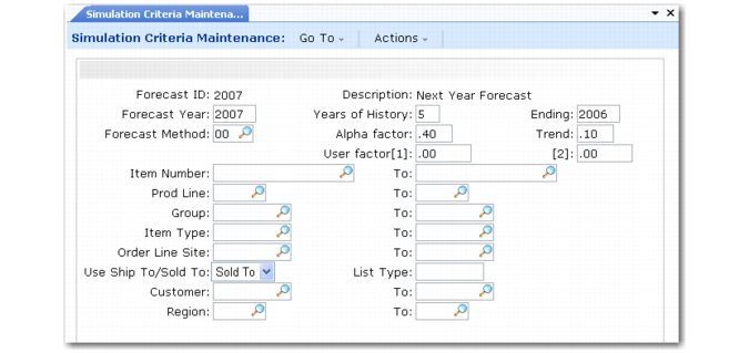
Simulation Criteria Maintenance (22.7.1)
Forecast Year
For a rolling forecast starting this month, this year must be identical to the ending year. See
Forecasting Horizon.
Years of History
Specify the number of years of shipment history to analyze, up to five years. The system reduces this number if there are no sales data for a given year.
Ending
Ending year must be the same as or earlier than the forecast year.
Forecast Method
Specify either a predefined forecast method (01–06) or your own forecast method.See
Forecast Methods.
Alpha factor, Trend, User factor [1] and [2]
Specify weighting factors used by the forecast method. See
Alpha and Trend Factors.
Item Number, Product Line, Group, Item Type
Use these fields to identify a single item or range of items for which to forecast.
Order Line Site
Specify the order line site on sales orders or ship-from site on a customer schedule, used to further define items to forecast.
Use Ship-To/Sold-To
Indicate whether the system selects sales history to analyze based on the customer’s ship-to or sold-to address.
Customer, Region, List Type
Use these fields to identify subsets of customers for which the system selects sales data to analyze.
Note: When you specify both Ship-To and Region as criteria for selecting sales history data, only permanent ship-to addresses—that is, those defined for customers in Financials—are in the selected region range.
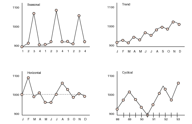
Demand Patterns
Sales history can contain four underlying patterns of demand. Forecasting methods quantify these patterns.
Demand Patterns
Pattern | Description | Example |
Trend | Sales quantities increase or decrease over time. | The growth pattern of a new product. |
Seasonal | Sales quantities fluctuate according to some seasonal factor, such as weather or the way a firm handles its operations. | Sales of soft drinks, which increase in the summer months. |
Cyclical | This pattern is similar to seasonal, but the length is greater than one year. The pattern does not repeat at constant intervals and is the hardest to predict. | The sale of houses. |
Horizontal | Sales quantities do not increase or decrease substantially. | A stable product with consistent demand. |
Demand Patterns shows examples of these demand patterns in graph format.
Demand Patterns
Forecast Methods
Forecast methods are identified by two-digit method numbers.
Method Numbers lists the forecast method numbers available.
Method Numbers
Method Number | Usage |
00 | Indicates that a forecast detail record was not generated by the system, but was created manually using the copy programs or using CIM interface. |
01–06 | Predefined forecast methods. |
07–50 | Reserved for QAD usage. |
51–99 | Use these numbers to identify your own forecasting methods. |
There are six predefined forecast methods, described in
Predefined Forecast Methods. You can create additional methods using User Forecast Method Maintenance (22.7.17).
Predefined Forecast Methods
Method # | Type | Description |
01 | Best Fit | Uses all predefined methods—02 through 06—and selects the results with the least mean absolute deviation. This is the default forecast method. |
02 | Double Moving Average | The simplest of the forecasting techniques. It uses a set of simple moving averages based on historical data and then computes another set of moving averages based on the first set. The moving averages are based on four months of data. This method produces a forecast that lags behind trend effects. |
03 | Double Exponential Smoothing | The most popular of the forecast techniques. It is similar to Double Moving Average, except that it uses the alpha factor to weigh the most recent sales data more heavily than the older sales data. This method produces a forecast that lags behind trends effects. |
04 | Winter’s Linear Exponential Smoothing | Produces results similar to Double Exponential Smoothing, but incorporates a seasonal/trend adjustment factor. This method can be used to forecast based on sales history containing both trends and seasonal patterns. Uses the trend and alpha factors. Requires two years of history. |
05 | Classic Decomposition | Recognizes three separate elements of demand patterns in sales history: trend, seasonal, and cyclical factors. See Demand Patterns for information about demand patterns. Classic Decomposition is usually the preferred method for forecasting seasonal, high-cost items. It requires at least two years of history. |
06 | Simple Regression | Also called the least squared method, this method analyzes the relationship between sales and time span to ensure that the forecast quantity is equally likely to be higher or lower than the actual quantity sold. Useful for products with a stable history, or horizontal demand pattern. |
Overview of Forecast Methods shows each of the predefined forecast methods and indicates the sales patterns they are typically used to quantify, the number of years of shipment history required for calculation, and whether they use alpha and trend factors.
Overview of Forecast Methods
| 01 | 02 | 03 | 04 | 05 | 06 |
Cyclical | | | | | Yes | |
Trend | | Lags | Lags | Yes | Yes | |
Seasonal | | | | Yes | Yes | |
Horizontal | | | | | | Yes |
Years of History | 1 | 1 | 1 | 2 | 2–3 | 1 |
Trend Factor | | | | Yes | | |
Alpha Factor | | | Yes | Yes | | |
Alpha and Trend Factors
Some forecast methods use alpha and trend factors to weight shipment history when calculating forecasts.
When method 03 or 04 is used to calculate forecasts, alpha factors determine the relative importance given to more recent sales history. For new products with rapidly changing sales quantities, you may want to enter an alpha value closer to one to give more weight to recent sales history. However, for products with long and stable sales histories, you might specify a smaller alpha value to produce smoother forecast results.
When method 04 is used to calculate forecasts, trend factors determine the relative weight given to sharp increases or decreases in sales history when calculating forecasts.
Alpha and Trend Factors shows the effects of alpha and trend factors on forecasting calculations. Alpha and trend values must be between zero and one.
Alpha and Trend Factors
Factor | Zero | One |
Alpha Factor | Equal weight on all history | Weighs recent history |
Trend Factor | Ignores sharp changes in history | Weighs heavily sharp changes in history |
Creating Additional Forecast Methods
Forecast methods identify the Progress program the system uses to calculate forecasts. Different programs employ different statistical methods.
You can create specialized forecast methods for the system to use in producing forecast quantities. User Forecast Method Maintenance (22.7.17) lets you add your forecast methods, in the form of Progress programs you supply, to the existing forecast methods.
The criteria template includes two variables that can be set to interact with your own forecast method: User factor1 and User factor2. These are reserved for your forecast methods and do not operate with any of the predefined methods.
For user-defined forecast methods:
• The name of the program must be ffcalcXX.p where XX is a forecast method number between 51 and 99.
• The Progress program must be written and accessible to the system before you can define the method number in User Forecast Method Maintenance.
• Your Progress program must use an array named calc[1–60] for the historical data input and an array named fcast[1–12] for the calculated output.
• Your Progress program must include the following files at the beginning of the program: fcalvar.i and ffvar.i.
Compare your forecast method program to the existing programs ffcalc[02–06].p, as needed.